FitzHugh–Nagumo model

FitzHugh-Nagumo model in phase space, with $a=0.7,b=0.8,\tau =12.5,R=0.1,I_{ext}=0.5$. The green line is the cubic nullcline and the red line is the linear nullcline. The black lines are integral curves.

Graph of v with parameters I=0.5, a=0.7, b=0.8, and τ=12.5

The FitzHugh–Nagumo model (FHN) describes a prototype of an excitable system (e.g., a neuron).

It is an example of a relaxation oscillator because, if the external stimulus $I_{\text{ext}}$ exceeds a certain threshold value, the system will exhibit a characteristic excursion in phase space, before the variables $v$ and $w$ relax back to their rest values.

This behaviour is a sketch for neural spike generations, with a short, nonlinear elevation of membrane voltage $v$, diminished over time by a slower, linear recovery variable $w$ representing sodium channel reactivation and potassium channel deactivation, after stimulation by an external input current.

The equations for this dynamical system read

${\dot {v}}=v-{\frac {v^{3}}{3}}-w+RI_{\rm {ext}}$

$\tau {\dot {w}}=v+a-bw.$

The FitzHugh–Nagumo model is a simplified 2D version of the Hodgkin–Huxley model which models in a detailed manner activation and deactivation dynamics of a spiking neuron.

In turn, the Van der Pol oscillator is a special case of the FitzHugh–Nagumo model, with $a=b=0$.

History

It was named after Richard FitzHugh (1922–2007) who suggested the system in 1961 and Jinichi Nagumo et al. who created the equivalent circuit the following year.

In the original papers of FitzHugh, this model was called Bonhoeffer–Van der Pol oscillator (named after Karl-Friedrich Bonhoeffer and Balthasar van der Pol) because it contains the Van der Pol oscillator as a special case for $a=b=0$. The equivalent circuit was suggested by Jin-ichi Nagumo, Suguru Arimoto, and Shuji Yoshizawa.

Qualitative analysis

Qualitatively, the dynamics of this system is determined by the relation between the three branches of the cubic nullcline and the linear nullcline.

The cubic nullcline is defined by ${\dot {v}}=0\leftrightarrow w=v-v^{3}/3+RI_{ext}$.

The linear nullcline is defined by ${\dot {w}}=0\leftrightarrow w=(v+a)/b$.

In general, the two nullclines intersect at one or three points, each of which is an equilibrium point. At large values of $v^{2}+w^{2}$, far from origin, the flow is a clockwise circular flow, consequently the sum of the index for the entire vector field is +1. This means that when there is one equilibrium point, it must be a clockwise spiral point or a node. When there are three equilibrium points, they must be two clockwise spiral points and one saddle point.

• If the linear nullcline pierces the cubic nullcline from downwards then it is a clockwise spiral point or a node.
• If the linear nullcline pierces the cubic nullcline from upwards in the middle branch, then it is a saddle point.

The type and stability of the index +1 can be numerically computed by computing the trace and determinant of its Jacobian:

$$(tr,\det )=(1-b/\tau -v^{2},(v^{2}-1)b/\tau +1/\tau )$$

The point is stable iff the trace is negative. That is, $v^{2}>1-b/\tau$.

The point is a spiral point iff $4\det -tr^{2}>0$. That is, $(\tau v^{2}-b-\tau )^{2}<4\tau$.

The limit cycle is born when a stable spiral point becomes unstable by Hopf bifurcation.

Only when the linear nullcline pierces the cubic nullcline at three points, the system has a separatrix, being the two branches of the stable manifold of the saddle point in the middle.

• If the separatrix is a curve, then trajectories to the left of the separatrix converge to the left sink, and similarly for the right.
• If the separatrix is a cycle around the left intersection, then trajectories inside the separatrix converge to the left spiral point. Trajectories outside the separatrix converge to the right sink. The separatrix itself is the limit cycle of the lower branch of the stable manifold for the saddle point in the middle. Similarly for the case where the separatrix is a cycle around the right intersection.
• Between the two cases, the system undergoes a homoclinic bifurcation.

Gallery figures: FitzHugh-Nagumo model, with $a=0.7,\tau =12.5,R=0.1$, and varying $b,I_{ext}$. (They are animated. Open them to see the animation.)

• 
  b = 0.8. The nullclines always intersect at one point. When the point is in the middle branch of the cubic nullcline, there is a limit cycle and an unstable clockwise spiral point.
• 
  b = 1.25. The limit cycle still exists, but for a smaller interval of I_ext. When there are three intersections in the middle, two of them are unstable spirals and one is an unstable saddle point.
• 
  b = 2.0. The limit cycle has disappeared, and instead we sometimes get two stable fixed points.
• 
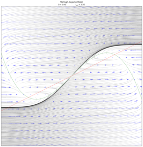  When $b=2,I_{ext}=3.5$, we can easily see the separatrix and the two basins of attraction by solving for the trajectories backwards in time.
• 
  When $b=2.0$, a homoclinic bifurcation event occurs around $I_{ext}=5.393$. Before the bifurcation, the stable manifold converges to the sink, and the unstable manifold escapes to infinity. After the event, the stable manifold converges to the sink on the right, and the unstable manifold converges to a limit cycle around the left spiral point.
• 
  After the homoclinic bifurcation. When $b=2.0,I_{ext}=5.45$, there is one stable spiral point on the left, and one stable sink on the right. Both branches of the unstable manifold converge to the sink. The upper branch of the stable manifold diverges to infinity. The lower branch of the stable manifold converges to a cycle around the spiral point. The limit cycle itself is unstable.

See also

• Autowave
• Biological neuron model
• Computational neuroscience
• Hodgkin–Huxley model
• Morris–Lecar model
• Reaction–diffusion
• Theta model
• Chialvo map

Further reading

• FitzHugh R. (1955) "Mathematical models of threshold phenomena in the nerve membrane". Bull. Math. Biophysics, 17:257—278
• FitzHugh R. (1961) "Impulses and physiological states in theoretical models of nerve membrane". Biophysical J. 1:445–466
• FitzHugh R. (1969) "Mathematical models of excitation and propagation in nerve". Chapter 1 (pp. 1–85 in H. P. Schwan, ed. Biological Engineering, McGraw–Hill Book Co., N.Y.)
• Nagumo J., Arimoto S., and Yoshizawa S. (1962) "An active pulse transmission line simulating nerve axon". Proc. IRE. 50:2061–2070.

External links

• FitzHugh–Nagumo model on Scholarpedia
• Interactive FitzHugh-Nagumo. Java applet, includes phase space and parameters can be changed at any time.
• Interactive FitzHugh–Nagumo in 1D. Java applet to simulate 1D waves propagating in a ring. Parameters can also be changed at any time.
• Interactive FitzHugh–Nagumo in 2D. Java applet to simulate 2D waves including spiral waves. Parameters can also be changed at any time.
• Java applet for two coupled FHN systems Options include time delayed coupling, self-feedback, noise induced excursions, data export to file. Source code available (BY-NC-SA license).

References

- ^ a b Sherwood, William Erik (2013), "FitzHugh–Nagumo Model", in Jaeger, Dieter; Jung, Ranu (eds.), Encyclopedia of Computational Neuroscience, New York, NY: Springer, pp. 1–11, doi:10.1007/978-1-4614-7320-6_147-1, ISBN 978-1-4614-7320-6, retrieved 2023-04-15
- ^ "Richard FitzHugh at the National Institute of Health - CHM Revolution". www.computerhistory.org. Archived from the original on 25 Mar 2023. Retrieved 2023-06-20.
- ^ FitzHugh, Richard (July 1961). "Impulses and Physiological States in Theoretical Models of Nerve Membrane". Biophysical Journal. 1 (6): 445–466. Bibcode:1961BpJ.....1..445F. doi:10.1016/S0006-3495(61)86902-6. PMC 1366333. PMID 19431309.
- ^ Nagumo, J.; Arimoto, S.; Yoshizawa, S. (October 1962). "An Active Pulse Transmission Line Simulating Nerve Axon". Proceedings of the IRE. 50 (10): 2061–2070. doi:10.1109/jrproc.1962.288235. ISSN 0096-8390. S2CID 51648050.
- ^ "SIAM: Obituaries: Jin-Ichi Nagumo". www.siam.org.